Lesson 6—Experimental Probability

Purpose

This lesson provides an informal and hands-on introduction to something called the geometric probability distribution, and to the use of programmed simulations to study probability. In doing these things, the lesson also introduces you to the while loop in Matlab.

Background

While Loops

The while loop is a mechanisms for repeating some group of statements a number of times, somewhat like the for loop. The difference between while and for is that for repeats the statements a fixed number of times, whereas while repeats them as long as some condition is true. A while loop is thus appropriate when you know what circumstances you want to keep repeating under, but not how long those circumstances might last, and a for loop is appropriate when you know in advance the number of times or set of values on which you want to repeat.

Section 5.3 of Attaway’s text discusses the while loop. The video on “The while loop” from the University of Edinburgh may also be helpful.

Geometric Distributions

Ask yourself how many times you will have to flip a coin before it comes up heads. You might get lucky, and have the coin produce heads on the first flip. Or you might get tails on the first flip and heads on the second, or two tails followed by heads on the third try, and so forth. In general, in order to need to flip the coin n times, you have to get tails on the first n-1 flips, and heads on the last. Intuitively, the probability of such a sequence of flips decreases as n increases. The graph of this probability versus n is an example of a geometric distribution.

More formally, suppose you are doing an experiment that can either succeed or fail, with the probability of success being p, and the probability of failure thus being 1-p. Different instances of the experiment are independent of each other, i.e., whether earlier instances succeeded or failed doesn’t influence the chances of the next instance succeeding or failing. Each instance of such an experiment is known as a Bernoulli trial. For example, the coin-flipping scenario described above is a sequence of Bernoulli trials (i.e., of experiments as described here) with the probability of success (getting heads) being 1/2, and the probability of failure thus being 1 - 1/2 or 1/2 also.

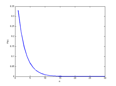
One can show that the probability of needing n Bernoulli trials in order to see the first success is p(1-p)^n-1. This relation between n and its probability is a geometric distribution. Probability distributions are often written as equations defining P(n), the probability of a number, n, occuring. In the case of geometric distributions, these equations are of the form P(n) = p(1-p)^n-1, for some given probability p.

As an example, here is a plot of a geometric distribution for p = 0.33:

Activity

Write a Matlab function that simulates multiple series of Bernoulli trials. Specifically, your function should take a probability, p, as its argument. It should simulate a large number (say, 1000) of series of Bernoulli trials with that probability. Each series of trials should continue until encountering the first success. Use Matlab’s random number generator (the rand function) to generate an outcome for each Bernoulli trial. During this simulation, the function should count the number of series that need 1 trial, 2 trials, 3 trials, etc. At the end of the simulation, your function should plot the counts versus the number of trials—this plot should show an approximately geometric distribution. Your function should return the count data from which it generated its plot (e.g., a vector of counts).

I expect that you will need to put some thought into the algorithm on which to base your script before you start to write it. To help start this thinking, we will use the first class meeting of this lesson for manual simulations similar to the one described above, using coins or dice as the source or randomness.

Extra Credit

The probabilities that users pass to your function should be numbers greater than 0 and less than or equal to 1. Write code in a separate script that prompts the user for a probability, checks to see if the response is in this range, and keeps asking for input until it is. Once the script has a valid probability, it should call your simulation function with that probability.

Both of the examples of while loops in the Edinburgh mini-lecture could arguably be done more elegantly with for loops. Show what the examples would look like using for loops instead of while loops. What, if anything, does this suggest to you about the relationship between while and for?

Follow-Up

I will grade this exercise in a face-to-face meeting with you. During this meeting I will look at your solution, ask you any questions I have about it, answer questions you have, etc. Please bring a written solution to the exercise to your meeting, as that will speed the process along.

Sign up for a meeting via Google calendar. If you worked in a group on this exercise, the whole group should schedule a single meeting with me. Please make the meeting 15 minutes long, and schedule it to finish before the end of the “Grade By” date above.