Research
Below is a description of the research projects that I have been fortunate to work on with great collaborators: nonlinear controllability, numerical solutions to optimal control problems, invariant manifolds in control theory, spectral graph theory, networked dynamical systems. Software packages that I use in my research are: SciPy Python, NetworkX, nauty, Armadillo C++
Controllability of Networked Dynamical Control Systems
NSF ECCS Grant No. 1509966,
1700578
Networks are a useful tool to model complex dynamic behavior in many branches of science and engineering. A networked dynamical system is a collection of dynamic units (e.g. ODEs) that are able to communicate and share information only locally with neighboring systems. The shared information between systems can affect the dynamics of each individual unit and the global dynamics. The communication network between units determines a graph (as in graph theory) and an inherent problem is to determine in graph-theoretic terms how the graph structure affects global dynamic behavior. From a control-theoretic standpoint, one is interested in altering the free dynamics of the networked system to achieve a desired global task such as state transfer, synchronization, sensoring, etc. A very practical problem is to understand how to properly select only a subset of the units to act as controlling agents that will be used to accomplish the desired task. Although the property of controllability is mathematically generic, many real-world networks possess a high-level of structure such as symmetries, regularity, tree structures, etc. Such structures impose significant constraints on the selection of agents to control the overall network.
- C.O. Aguilar, B. Gharesifard, Laplacian controllability classes for threshold graphs, Linear Algebra and Its Applications, Vol. 471, pp. 575-586, 2015. (journal version)
- C.O. Aguilar, B. Gharesifard, Graph controllability classes for the Laplacian leader-follower dynamics, IEEE Transactions on Automatic Control, Vol. 60, No. 6, pp. 1611-1623, 2015. (journal version)
- C.O. Aguilar, B. Gharesifard, Almost equitable partitions and new necessary conditions for network controllability, Automatica, Vol. 80, pp. 25-31, 2017. (journal version)
- C.O. Aguilar, Joon-yeob Lee, Eric Piato, Barbara J. Schweitzer, Spectral characterizations of anti-regular graphs, Linear Algebra and Its Applications, Vol. 557, pp. 84-104, 2018. (journal version)
- C.O. Aguilar, Strongly uncontrollable network topologies, IEEE Transactions on Control of Network Systems, accepted, 2019.(journal version)
- C.O. Aguilar, M. Ficarra, N. Schurman, B. Sullivan, The role of the anti-regular graph in the spectral analysis of threshold graphs, Linear Algebra and Its Applications, Vol. 588, pp. 210-223, 2020. (journal version)
Hamilton-Jacobi PDEs
\[ \frac{\partial V}{dt} + H(x,\nabla_x V) = 0 \] Hamilton-Jacobi equations are nonlinear PDEs arising in a broad range of integral minimization problems in optimal control, computer vision, geometric optics, and classical mechanics. The notion of viscosity solutions has been developed to settle the problem of existence and uniqueness of solutions to these nonlinear PDEs. In control theory, HJ PDEs arise in the problem of controlling an ODE \begin{align*} \dot{y}(s) &= f(y(s), u(s))\\ y(t) &= x \end{align*} so as to minimize an integral cost \[ J_t(x, u(\cdot)) = \int_t^T L(y(s),u(s))\,ds + g(y(T)) \] over all measurable control functions u(s). The value function \[ V(x,t):=\inf_{u(\cdot)} J_t(x,u(\cdot)) \] for the minimization problem satisfies a HJ PDE for the Hamiltonian function \[ H(x,p):=\min_u\{ f(x,u)\cdot p + L(x,u)\} \] In the literature, this HJ PDE is usually referred to as a Hamilton-Jacobi-Bellman (HJB) PDE due to its relation with the method of dynamic programming pioneered by Richard Bellman. Using a level set method, a Cauchy-Kowalevski technique, and the idea of patchy vector fields, we developed a numerical method to compute solutions to the HJB PDE. Below is a sample of the results of the method via the animation of the propagation of the level sets of the value function for the classical cart-pendulum system and a 3D cubic polynomial system with two control inputs.
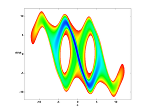
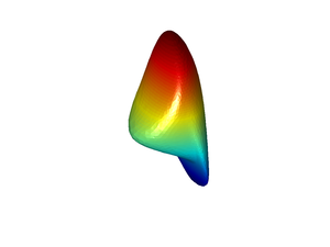
Both animations show the nonlinearity of HJ PDEs: self-intersection of the level sets and the formation of cusps on the level sets. In both cases, the value function looses differentiability but remains Lipschitz continuous. Possible projects in the future include developing robust numerical algorithms to deal with the aformentioned nonlinear effects and the presence of fast and slow dynamics. Another issue of interest involves the construction and/or incorporation of reliable adaptive algorithms to describe the local geometry of the level sets such as nearest neighbors information.
- C.O. Aguilar, A.J. Krener, High-order numerical solutions to Bellman's equation of optimal control, Proceedings of the American Control Conference, 2012, pp. 1832--1837. (proceedings version)
- C.O. Aguilar, A.J. Krener, Numerical solutions to the Bellman equation of optimal control, Journal of Optimization Theory and Applications, Vol. 160, No. 2, pp. 527-552, 2014. (journal version)
Periodic Center Manifolds
Invariant manifolds provide crucial insight into the overall qualitative behavior of a dynamical system. For example, an important feature of invariant manifolds is the simplification resulting from reduction of dimension as they organize the dynamics into smaller regions of the configuration space. Recently, there has been an active effort in developing numerical methods to compute (un)stable invariant manifolds of vector fields using geodesic level sets, BVP continuation of trajectories, computation of ``fat'' trajectories, and PDE formulations. The computation of center manifolds has received far less attention partially due to the subtle properties regarding existence and regularity of center manifolds. In control theory, the need to compute a center manifold arises in the problem of stabilizing a reference trajectory of the configuration variables. Through center manifold reduction, the trajectory stabilization problem can be solved by computing the solution φ to the invariant manifold PDE \[ \frac{\partial\varphi}{dw}(w)s(w) = f(\varphi(w),w) \] for the coupled ODEs \begin{align*} \dot{z} &= f(z,w)\\ \dot{w} &= s(w). \end{align*} The \(w\)-dynamics act like a forcing term in the z-dynamics and generate the desired reference trajectory to be stabilized. When the \(w\)-dynamics are 2-dimensional and neutrally stable, and the \(z\)-dynamics are hyperbolic, the invariant (center) manifold is generated by a real analytic one-parameter family of periodic trajectories. We developed a BVP continuation algorithm to compute the center manifold determined by the graph of \(\varphi\). Our work naturally lead to an investigation of extending our algorithm to higher-dimensional forcing terms. A future project is to extend the BVP continuation algorithm to isochronous forcing terms that possess a first integral and a natural choice of these systems are Hamiltonian isochronous systems.
- C.O. Aguilar, A.J. Krener, Piecewise smooth solutions to the nonlinear output regulation PDE, Proc. American Control Conference , 2011, pp. 1426-1427. (proceedings version)
- C.O. Aguilar, On the existence and uniqueness of solutions to the output regulator equations for periodic exosystems, Systems and Control Letters, 61, 702-706, 2012. (journal version)
- C.O. Aguilar, A.J. Krener, Patchy solution of a Francis-Byrnes-Isidori partial differential equation, International Journal of Robust and Nonlinear Control, Vol. 23, No. 9, pp. 1046-1061, 2013. (journal version)
Nonlinear Controllability
Given the controlled differential equation \begin{align*} \dot{x} &= f(x,u)\\ x(0) &= x_0 \end{align*} and a positive time \(T\), the reachable set \(R(T)\) consists of all the final states \(x(T)\) obtained by following the trajectories of the above control system as one varies the control function \(u(t)\) over some prescribed set of functions. The vector field \(f(x,u)\) determines the allowable infinitesimal motions from the point \(x\) and usually these are a strict subset of the full tangent space at \(x\). The classic example in control theory is parallel parking of a vehicle. At an initial configuration \(x\) assumed to be parallel with the curb, one can move only in a direction parallel with the curb and along directions tangent to a circle determined by the turning radius. At such an initial configuration, one cannot move in a direction perpendicular to the curb. However, as is common experience, by switching between these two allowable directions, it is possible to move the vehicle in such a way that its final position is a perpendicular shift of its initial condition. My work in the area of controllability centers on the notion of small-time local controllability (STLC). As part of my PhD dissertation, I considered the STLC property for a class of polynomial control-affine systems and determined a feedback invariant sufficient condition for STLC using Butcher rooted trees. It would be interesting to extend this work and develop a complete feedback invariant STLC characterization for these polynomial systems.
- C.O. Aguilar, Local controllability of affine distributions Ph.D. thesis, Queen's University, defended Dec 2009.
- C.O. Aguilar and A.D. Lewis, Small-time local controllability for a class of homogeneous systems, SIAM Journal on Control and Optimization, Vol. 50, No. 3, pp. 1502-1517, 2012. (journal version)
- C.O. Aguilar, Local controllability of control-affine systems with quadratic drift and constant control-input vector fields, Proc. 51th IEEE Conf. Decision and Control, pp. 1877--1882, 2012. ( proceedings version)